Forelesning 3: Statistisk analyse

I denne forelesningen skal vi se på statistisk analyse og hvordan vi kan bruke data til å lage modeller.

• gjøre statistiske operasjoner på data (pandas og numpy)

• tolke statistiske størrelser og visualiseringer (som boksplott)

• gjøre og tolke regresjon (numpy)

import pandas as pd
import numpy as np
import matplotlib.pyplot as plt
import seaborn as sns

Statistiske operasjoner

konsentrasjoner = [0.1, 0.2, 0.5, 0.5]
print(np.std(konsentrasjoner,ddof = 1))

0.20615528128088303

pandakons = pd.Series(konsentrasjoner)
print(pandakons.std())

0.20615528128088303

df = pd.read_csv("https://www.uio.no/studier/emner/matnat/ifi/IN-KJM1900/h20/datafiler/vin.csv")
df.head()

	fixed acidity	volatile acidity	citric acid	residual sugar	chlorides	free sulfur dioxide	total sulfur dioxide	density	pH	sulphates	alcohol	quality
0	7.4	0.70	0.00	1.9	0.076	11.0	34.0	0.9978	3.51	0.56	9.4	5
1	7.8	0.88	0.00	2.6	0.098	25.0	67.0	0.9968	3.20	0.68	9.8	5
2	7.8	0.76	0.04	2.3	0.092	15.0	54.0	0.9970	3.26	0.65	9.8	5
3	11.2	0.28	0.56	1.9	0.075	17.0	60.0	0.9980	3.16	0.58	9.8	6
4	7.4	0.70	0.00	1.9	0.076	11.0	34.0	0.9978	3.51	0.56	9.4	5

pH = df["pH"]
snitt = pH.mean()
avvik = pH.std()
print(f"pH i vinene er {snitt:.2f} +- {avvik:.2f}")

pH i vinene er 3.31 +- 0.15

med = pH.median()
med

3.31

Q1, Q2, Q3 = pH.quantile([0.25, 0.5, 0.75])
IQR = Q3 - Q1
print(f"pH i vinene er {Q2:.2f} +- {IQR:.2f}")

pH i vinene er 3.31 +- 0.19

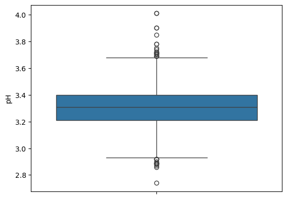
sns.boxplot(data = df, y = "pH")

<Axes: ylabel='pH'>

Regresjon

Temperatur (°C)	NH\(_3\), løselighet (g/100 mL H\(_2\)O)	NaCl, Løselighet (g/100 mL H\(_2\)O)
0	88.5	35.7
20	56.0	35.9
40	34.0	36.4
60	20.0	37.1
80	11.0	38.0
100	7.0	39.2

T = [0, 20, 40, 60, 80, 100]
NaCl = [35.7, 35.9, 36.4, 37.1, 38, 39.2]

a, b = np.polyfit(T, NaCl, 1)

x = np.linspace(0,120,10000)
y = a*x + b

plt.title("Løselighet av NaCl")
plt.plot(x, y, label = "Modell")
plt.scatter(T, NaCl, label = "Datapunkter", color = "firebrick")
plt.xlabel("Temperatur (C)")
plt.ylabel("Løselighet i g/100 mL")
plt.legend()
plt.show()